Electrostatic Field Between Two Intersecting Grounded Planes

Consider two infinite grounded metal planes with an angle $\alpha$ between them, as shown in the following figure. A point charge $Q$ is located at $(r_0,{\varphi }_0,0)$ in cylindrical coordinates, where $0<{\varphi }_0<\alpha$. Determine the electric potential in angle domain.

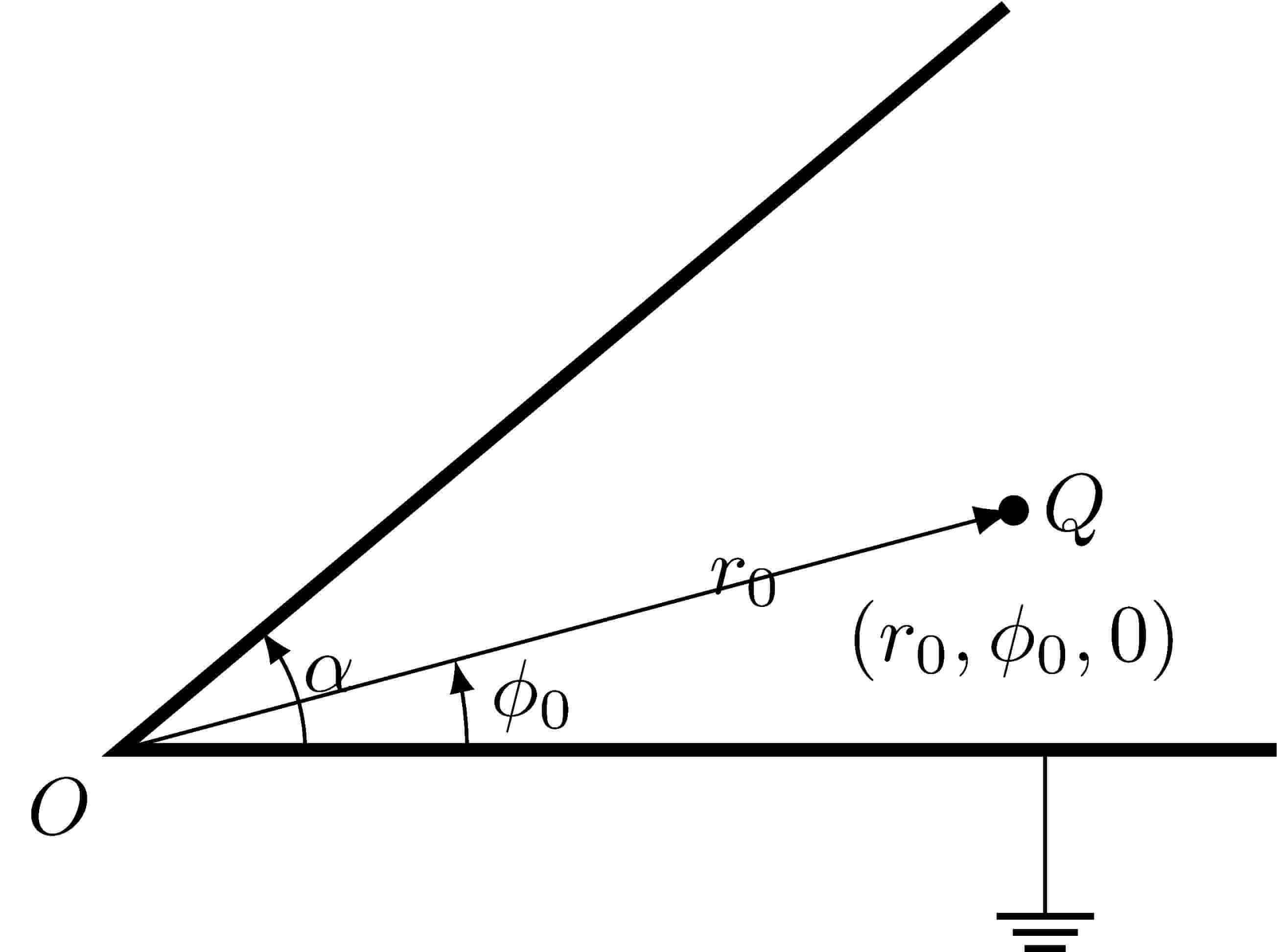
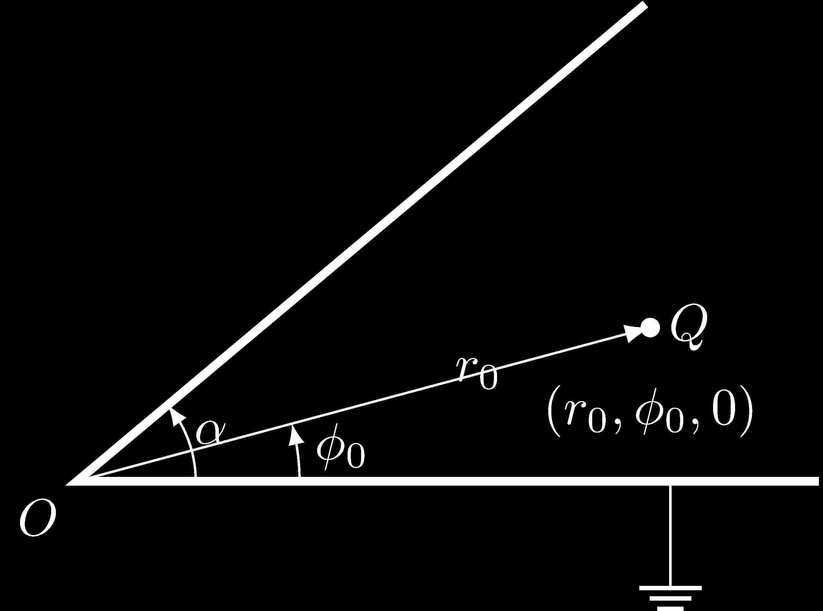Figure 1: Diagram of the problem

As a classical problem in electrodynamics, I believe most people have encountered it. This problem is extraordinary easy when $\alpha =\pi /n,n\in {\mathbb{Z}}^{+}$. But what about $\alpha \ne \pi /n$? It’s rare to see textbooks discussing this problem. Next, I’ll solve it with method of separation of variables and expand upon it.

In fact, this post was completed when I was a sophomore in college (2021). I am just reposting it this time, please see here. In addition, I also answered one of the key integrals on Zhihu, please see here.

1. Problem with Dirichlet boundary condition

1.1. Special case: $\alpha =\pi /n$

If $\alpha =\pi /n$, the system exhibits a high degree of symmetry, we can solve it using the method of images. Please see the following examples:

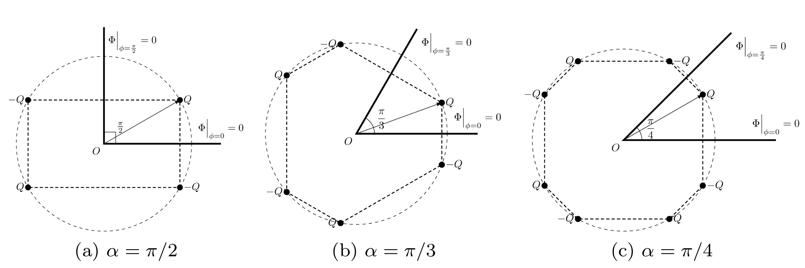
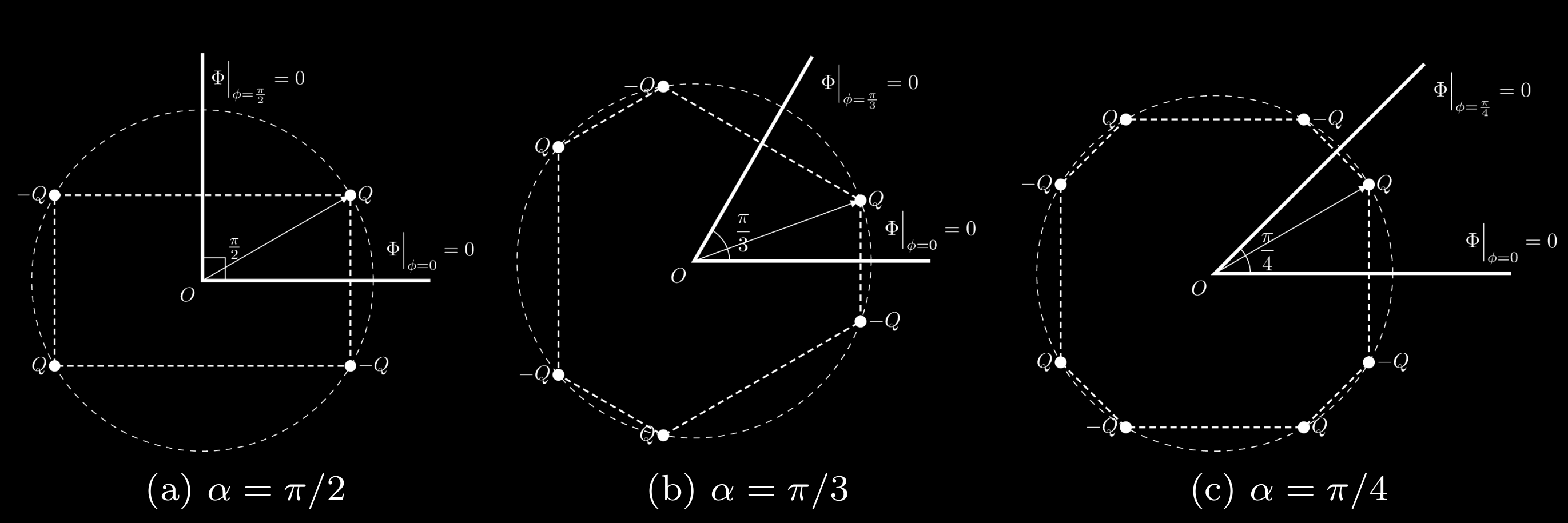Figure 2: The positions of the charge $Q$ and image charges for $n=2,3,4$ with Dirichlet boundary condition.

Obviously, the number of image charges is $2n-1$. The electric potential in angle domain can be obtained immediately,

$$\begin{array}{}\text{(1)}& \mathrm{\Phi }(r,\varphi ,z)=\frac{Q}{4\pi {ϵ}_0}\sum _{i=1}^{2n}\frac{(-1{)}^{n+1}}{|\mathbf{r}-{\mathbf{r}}_i|},\end{array}$$

where ${\mathbf{r}}_i=r_0{\mathbf{e}}_r+{\varphi }_i{\mathbf{e}}_{\varphi }$ and

$$\begin{array}{}\text{(2)}& {\varphi }_i=\left[\frac{i}{2}\right]\frac{2\pi }{n}+(-1{)}^{i+1}{\varphi }_0,(i=1,2,\dots ,2n).\end{array}$$

Or we can rewrite $\text{(1)}$ as

$$\begin{array}{}\text{(3)}& \mathrm{\Phi }(r,\varphi ,z)=\frac{Q}{4\pi {ϵ}_0}\sum _{i=1}^{2n}\frac{(-1{)}^{i+1}}{\sqrt{r^2+r_0^2+z^2-2r{r}_0\cos (\varphi -{\varphi }_i)}}.\end{array}$$

1.2. General case: $\alpha$ can be any value

When $\alpha$ is arbitrary, the system no longer possesses a definite high degree symmetry, rendering the method of images ineffective. In such cases, solving the Poisson’s equation directly becomes the most straightforward approach,

$$\begin{array}{}\text{(4)}& {\mathrm{\nabla }}^2\mathrm{\Phi }=-\frac{\rho }{{ϵ}_0}=-\frac{Q}{{ϵ}_0}\delta (\mathbf{r}-{\mathbf{r}}_0).\end{array}$$

In cylindrical coordinates, this equation with Dirichlet boundary conditions (because the metal planes are grounded) can be expressed as:

$$\begin{array}{}\text{(5)}& \{\begin{array}{l}{\displaystyle \frac{1}{r}\frac{\partial }{\partial r}\left(r\frac{\partial \mathrm{\Phi }}{\partial r}\right)+\frac{1}{r^2}\frac{{\partial }^2\mathrm{\Phi }}{\partial {\varphi }^2}+\frac{{\partial }^2\mathrm{\Phi }}{\partial z^2}=-\frac{Q}{{ϵ}_0{r}_0}\delta (r-r_0)\delta (\varphi -{\varphi }_0)\delta (z),}\\ {\displaystyle {\mathrm{\Phi }\phantom{\int }|}_{\varphi =0}={\mathrm{\Phi }\phantom{\int }|}_{\varphi =\alpha }=0.}\end{array}\end{array}$$

Solving this problem is not easy, we can use the method of separation of variables. But we still need to approach it step by step.

1.2.1. Find the eigenfunctions

Suppose the solution $\mathrm{\Phi }$ can be written as $\mathrm{\Phi }=R(r)\psi (\varphi )Z(z)$, if $\mathbf{r}\ne {\mathbf{r}}_0$, the Poisson’s equation becomes Laplace’s equation:

$$\psi Z\frac{{\mathrm{d}}^{2}R}{\mathrm{d}{r}^2}+\frac{Z\psi }{r}\frac{\mathrm{d}R}{\mathrm{d}r}+\frac{RZ}{r^2}\frac{{\mathrm{d}}^2\psi }{\mathrm{d}{\varphi }^2}+R\psi \frac{{\mathrm{d}}^{2}Z}{\mathrm{d}{z}^2}=0.$$

Multiplying each term by $r^2/R\psi Z$ and rearranging appropriately, the equation becomes:

$$\frac{r^2}{R}\frac{{\mathrm{d}}^{2}R}{\mathrm{d}{r}^2}+\frac{r}{R}\frac{\mathrm{d}R}{\mathrm{d}r}+r^2\frac{1}{Z}\frac{{\mathrm{d}}^{2}Z}{\mathrm{d}{z}^2}=-\frac{1}{\psi }\frac{{\mathrm{d}}^2\psi }{\mathrm{d}{\varphi }^2}.$$

The right hand side is a function of $\varphi$, while the left hand side is a function of $r$ and $z$. So both sides must equal the same constant, denoted as $m^2$. Therefore,

$$-\frac{1}{\psi }\frac{{\mathrm{d}}^2\psi }{\mathrm{d}{\varphi }^2}=m^2⟹\psi (\varphi )=A\cos m\varphi +B\sin m\varphi .$$

With boundary condition ${\psi \phantom{\int }|}_{\varphi =0}={\psi \phantom{\int }|}_{\varphi =\alpha }=0$, we have

$$\begin{array}{}\text{(6)}& \psi (\varphi )=\sin \left(\frac{k\pi }{\alpha }\varphi \right),m=\frac{k\pi }{\alpha }(k=1,2,\dots ).\end{array}$$

Similarly, we have

$$\frac{1}{R}\frac{{\mathrm{d}}^{2}R}{\mathrm{d}{r}^2}+\frac{1}{rR}\frac{\mathrm{d}R}{\mathrm{d}r}-\frac{m^2}{r^2}=-\frac{1}{Z}\frac{{\mathrm{d}}^{2}Z}{\mathrm{d}{z}^2}.$$

The right hand side is a function of $z$, while the left hand side is a function of $r$. Obviously, both sides must equal the same constant too. Note the boundary condition ${\mathrm{\Phi }\phantom{\int }|}_{z\to \pm \mathrm{\infty }}=0$, so the constant must be ${\mu }^2$. Therefore,

$$-\frac{1}{Z}\frac{{\mathrm{d}}^{2}Z}{\mathrm{d}{z}^2}={\mu }^2⟹Z=A\sin \left(\mu z\right)+B\cos \left(\mu z\right).$$

Note that $\mathrm{\Phi }(z=0)\ne 0$ and $\cos \left(\mu z\right)$ is an even function, so we can assume $\mu >0$, then

$$\begin{array}{}\text{(7)}& Z(z)=\cos \left(\mu z\right),\text{(}\mu \text{ is continuous, }\mu >0\text{)}\end{array}$$

Finally, $R(r)$ satisfies the following equation:

$$\frac{{\mathrm{d}}^{2}R}{\mathrm{d}{r}^2}+\frac{1}{r}\frac{\mathrm{d}R}{\mathrm{d}r}-({\mu }^2+\frac{m^2}{r^2})R=0.$$

Let $x=\mu r$, it becomes

$$\frac{{\mathrm{d}}^{2}R}{\mathrm{d}{x}^2}+\frac{1}{x}\frac{\mathrm{d}R}{\mathrm{d}x}-(1+\frac{m^2}{x^2})R=0.$$

This is the standard $m$-order modified Bessel equation, and its solution is

$$R(r)=A{I}_m(x)+B{K}_m(x)=A{I}_m(\mu r)+B{K}_m(\mu r),$$

where $I_m(x)$ and $K_m(x)$ are the modified Bessel functions of the first and second kind respectively. They have the following properties:

$$\begin{array}{c}{I}_m(x)\stackrel{x\to 0}{\to }\frac{1}{\mathrm{\Gamma }(m+1)}{\left(\frac{x}{2}\right)}^m,I_m(x)\stackrel{x\to \mathrm{\infty }}{\to }\frac{1}{\sqrt{2\pi x}}{e}^x[1+\mathcal{O}\left(\frac{1}{x}\right)],\\ K_m(x)\underset{m\ne 0}{\overset{x\to 0}{\to }}\frac{\mathrm{\Gamma }(m)}{2}{\left(\frac{2}{x}\right)}^m,K_m(x)\stackrel{x\to \mathrm{\infty }}{\to }\sqrt{\frac{\pi }{2x}}{e}^{-x}[1+\mathcal{O}\left(\frac{1}{x}\right)].\end{array}$$

Since $r\in (0,\mathrm{\infty })$, to make the electric potential not divergent and continuous except for the original point, $R(r)$ needs to be divided into two parts by $r$:

$$\begin{array}{}\text{(8)}& R(r)=\{\begin{array}{l}{I}_m(\mu r),r\in (0,r_0)\\ K_m(\mu r),r\in (r_0,\mathrm{\infty })\end{array}\end{array}$$

Combine the results $\text{(6)}$,$\text{(7)}$,$\text{(8)}$, we find the eigenfunctions of the original problem,

$${\mathrm{\Phi }}_{k\mu }(r,\varphi ,z)=\left\{\begin{array}{l}{\displaystyle I_{k\pi /\alpha }(\mu r)\cos \left(\mu z\right)\sin \left(\frac{k\pi }{\alpha }\varphi \right),r\in (0,r_0)}\\ {\displaystyle K_{k\pi /\alpha }(\mu r)\cos \left(\mu z\right)\sin \left(\frac{k\pi }{\alpha }\varphi \right),r\in (r_0,\mathrm{\infty })}\end{array}\right\},(k\in {\mathbb{Z}}^{+};\mu \text{ is continuous , }\mu >0)$$

So the general solution can be expressed as linear superposition of these eigenfunctions,

$$\begin{array}{}\text{(9)}& \begin{array}{rl}\mathrm{\Phi }(r,\varphi ,z)& =\sum _{k=1}^{\mathrm{\infty }}{\int }_0^{\mathrm{\infty }}\mathrm{d}\mu a_{k\mu }{\mathrm{\Phi }}_{k\mu }(r,\varphi ,z)\\ & =\{\begin{array}{ll}{\displaystyle \sum _{k=1}^{\mathrm{\infty }}{\int }_0^{\mathrm{\infty }}\mathrm{d}\mu A_{k\mu }{I}_{k\pi /\alpha }(\mu r)\cos \left(\mu z\right)\sin \left(\frac{k\pi }{\alpha }\varphi \right),}& r<r_0\\ {\displaystyle \sum _{k=1}^{\mathrm{\infty }}{\int }_0^{\mathrm{\infty }}\mathrm{d}\mu B_{k\mu }{K}_{k\pi /\alpha }(\mu r)\cos \left(\mu z\right)\sin \left(\frac{k\pi }{\alpha }\varphi \right),}& r>r_0\end{array}\end{array}\end{array}$$

1.2.2. Calculate the coefficients

Even though we get $\text{(9)}$, it’s not the final result we want. Because it still has undetermined coefficients $A_{k\mu },B_{k\mu }$. Note that we have two conditions we haven’t used yet,

1. The electric potential should be continuous at $\mathbf{r}={\mathbf{r}}_0$;
2. The electric potential satisfies the Poisson’s equation, and the right side of the Poisson equation is the Dirac function.

First let us consider continuity, we can get

$$\sum _{k=1}^{\mathrm{\infty }}{\int }_0^{\mathrm{\infty }}\mathrm{d}\mu A_{k\mu }{I}_{k\pi /\alpha }(\mu r_0)\cos \left(\mu z\right)\sin \left(\frac{k\pi }{\alpha }\varphi \right)=\sum _{k=1}^{\mathrm{\infty }}{\int }_0^{\mathrm{\infty }}\mathrm{d}\mu B_{k\mu }{K}_{k\pi /\alpha }(\mu r_0)\cos \left(\mu z\right)\sin \left(\frac{k\pi }{\alpha }\varphi \right).$$

Integrate $z$ on both sides and use

$$\begin{array}{}\text{(10)}& \delta (\mu )=\frac{1}{2\pi }{\int }_{-\mathrm{\infty }}^{\mathrm{\infty }}\mathrm{d}z{e}^{i\mu z}=\frac{1}{2\pi }{\int }_{-\mathrm{\infty }}^{\mathrm{\infty }}\mathrm{d}z\cos \left(\mu z\right).\end{array}$$

It becomes

$$\sum _{k=1}^{\mathrm{\infty }}{A}_{k\mu }{I}_{k\pi /\alpha }(\mu r_0)\sin \left(\frac{k\pi }{\alpha }\varphi \right)=\sum _{k=1}^{\mathrm{\infty }}{B}_{k\mu }{K}_{k\pi /\alpha }(\mu r_0)\sin \left(\frac{k\pi }{\alpha }\varphi \right).$$

Due to the orthogonality of $\sin \left(k\pi \varphi /\alpha \right)$ in $\varphi \in (0,\alpha )$, the corresponding coefficients must be equal, so we obtain the first relation:

$$\begin{array}{}\text{(11)}& A_{k\mu }{I}_{k\pi /\alpha }(\mu r_0)=B_{k\mu }{K}_{k\pi /\alpha }(\mu r_0).\end{array}$$

Next, using the second condition and substituting the general solution into Poisson’s equation, we can get

$$\begin{array}{c}\sum _{k=1}^{\mathrm{\infty }}{\int }_0^{\mathrm{\infty }}\mathrm{d}\mu a_{k\mu }[\sin \left(\frac{k\pi \varphi }{\alpha }\right)\cos \left(\mu z\right)\frac{{\mathrm{d}}^{2}R}{\mathrm{d}{r}^2}+\frac{\sin \left(k\pi \varphi /\alpha \right)\cos \left(\mu z\right)}{r}\frac{\mathrm{d}R}{\mathrm{d}r}+\frac{R\cos \left(\mu z\right)}{r^2}\frac{{\mathrm{d}}^2\sin \left(k\pi \varphi \right)}{\mathrm{d}{\varphi }^2}\hfill \\ \hfill +R\sin \left(\frac{k\pi \varphi }{\alpha }\right)\frac{{\mathrm{d}}^2\cos \left(\mu z\right)}{\mathrm{d}{z}^2}]=-\frac{Q}{{ϵ}_0{r}_0}\delta (r-r_0)\delta (\varphi -{\varphi }_0)\delta (z).\end{array}$$

Note that $\mathrm{d}R/\mathrm{d}r$ is discontinuous at $r=r_0$, we can integrate the neighborhood of $r_0$ to cancel the $\delta (r-r_0)$,

$$\underset{\delta \to 0}{lim}\sum _{k=1}^{\mathrm{\infty }}{\int }_0^{\mathrm{\infty }}\mathrm{d}\mu {\int }_{r_0-\delta }^{r_0+\delta }\mathrm{d}r{a}_{k\mu }[\sin \left(\frac{k\pi \varphi }{\alpha }\right)\cos \left(\mu z\right)\frac{{\mathrm{d}}^{2}R}{\mathrm{d}{r}^2}]=-\frac{Q}{{ϵ}_0{r}_0}\delta (\varphi -{\varphi }_0)\delta (z).$$

Similarly, integrate $z$ on both sides,

$$\begin{array}{rl}& \underset{\delta \to 0}{lim}\sum _{k=1}^{\mathrm{\infty }}{\int }_0^{\mathrm{\infty }}\mathrm{d}\mu {\int }_{r_0-\delta }^{r_0+\delta }\mathrm{d}r{a}_{k\mu }\{\sin \left(\frac{k\pi \varphi }{\alpha }\right)[{\int }_{-\mathrm{\infty }}^{\mathrm{\infty }}\mathrm{d}z\cos \left(\mu z\right)]\frac{{\mathrm{d}}^{2}R}{\mathrm{d}{r}^2}\}\\ =& \underset{\delta \to 0}{lim}\sum _{k=1}^{\mathrm{\infty }}{\int }_0^{\mathrm{\infty }}\mathrm{d}\mu {\int }_{r_0-\delta }^{r_0+\delta }\mathrm{d}r2\pi a_{k\mu }\delta (\mu )[\sin \left(\frac{k\pi \varphi }{\alpha }\right)\frac{{\mathrm{d}}^{2}R}{\mathrm{d}{r}^2}]\\ =& \underset{\delta \to 0}{lim}\sum _{k=1}^{\mathrm{\infty }}{\int }_{r_0-\delta }^{r_0+\delta }\mathrm{d}r\pi a_{k\mu }[\sin \left(\frac{k\pi \varphi }{\alpha }\right)\frac{{\mathrm{d}}^{2}R}{\mathrm{d}{r}^2}]=-\frac{Q}{{ϵ}_0{r}_0}\delta (\varphi -{\varphi }_0).\end{array}$$

Then, with the orthogonality of $\sin \left(k\pi \varphi /\alpha \right)$, multiply both sides by $\sin \left(k^{\prime }\pi \varphi /\alpha \right)$ and integrate $\varphi$,

$$\begin{array}{rl}\underset{\delta \to 0}{lim}{\int }_{r_0-\delta }^{r_0+\delta }\frac{\alpha \pi a_{k\mu }}{2}\frac{{\mathrm{d}}^{2}R}{\mathrm{d}{r}^2}\mathrm{d}r& =-\frac{Q}{{ϵ}_0{r}_0}\sin \left(\frac{k\pi {\varphi }_0}{\alpha }\right)\\ & =\frac{\alpha \pi }{2}(B_{k\mu }\frac{\mathrm{d}{K}_{k\pi /\alpha }(\mu r_0)}{\mathrm{d}r}-A_{k\mu }\frac{\mathrm{d}{I}_{k\pi /\alpha }(\mu r_0)}{\mathrm{d}r}).\end{array}$$

It turns out to be the second relation

$$\begin{array}{}\text{(12)}& A_{k\mu }{I}_{k\pi /\alpha }^{\prime }(\mu r_0)-B_{k\mu }{K}_{k\pi /\alpha }^{\prime }(\mu r_0)=\frac{2Q}{\mu \alpha {ϵ}_0{r}_0\pi }\sin \left(\frac{k\pi {\varphi }_0}{\alpha }\right).\end{array}$$

Combining $\text{(11)}$ and $\text{(12)}$, we can get the coefficient $A_{k\mu },B_{k\mu }$

$$\begin{array}{}\text{(13)}& \{\begin{array}{l}{\displaystyle A_{k\mu }=\frac{2Q}{\mu \alpha {ϵ}_0{r}_0\pi }\sin \left(\frac{k\pi {\varphi }_0}{\alpha }\right)\frac{K_{k\pi /\alpha }(\mu r_0)}{K_{k\pi /\alpha }(\mu r_0)I_{k\pi /\alpha }^{\prime }(\mu r_0)-K_{k\pi /\alpha }^{\prime }(\mu r_0)I_{k\pi /\alpha }(\mu r_0)},}\\ {\displaystyle B_{k\mu }=\frac{2Q}{\mu \alpha {ϵ}_0{r}_0\pi }\sin \left(\frac{k\pi {\varphi }_0}{\alpha }\right)\frac{I_{k\pi /\alpha }(\mu r_0)}{K_{k\pi /\alpha }(\mu r_0)I_{k\pi /\alpha }^{\prime }(\mu r_0)-K_{k\pi /\alpha }^{\prime }(\mu r_0)I_{k\pi /\alpha }(\mu r_0)}.}\end{array}\end{array}$$

But that is not enough, we can simplify these expressions further with the Wrońskian of the modified Bessel functions:

$$\begin{array}{}\text{(14)}& W[K_m(x),I_m(x)]=K_m(x)I_m^{\prime }(x)-K_m^{\prime }(x)I_m(x)=\frac{1}{x}.\end{array}$$

So

$$K_{k\pi /\alpha }(\mu r_0)I_{k\pi /\alpha }^{\prime }(\mu r_0)-K_{k\pi /\alpha }^{\prime }(\mu r_0)I_{k\pi /\alpha }(\mu r_0)=\frac{1}{\mu r_0},$$

where the prime means the derivative with respect to $\mu r_0$. The finally results of $A_{k\mu },B_{k\mu }$ are

$$\begin{array}{}\text{(15)}& \{\begin{array}{l}{\displaystyle A_{k\mu }=\frac{2Q}{\alpha {ϵ}_0\pi }\sin \left(\frac{k\pi {\varphi }_0}{\alpha }\right)K_{k\pi /\alpha }(\mu r_0),}\\ {\displaystyle B_{k\mu }=\frac{2Q}{\alpha {ϵ}_0\pi }\sin \left(\frac{k\pi {\varphi }_0}{\alpha }\right)I_{k\pi /\alpha }(\mu r_0).}\end{array}\end{array}$$

1.2.3. Final result

After obtaining the coefficients $A_{k\mu },B_{k\mu }$, integrating $\text{(9)}$ and $\text{(15)}$, we can write the final solution of the original problem:

$$\mathrm{\Phi }(r,\varphi ,z)=\{\begin{array}{l}{\displaystyle \sum _{k=1}^{\mathrm{\infty }}{\int }_0^{\mathrm{\infty }}\mathrm{d}\mu \frac{2Q}{\alpha {ϵ}_0\pi }\sin \left(\frac{k\pi {\varphi }_0}{\alpha }\right)K_{k\pi /\alpha }(\mu r_0)I_{k\pi /\alpha }(\mu r)\cos \left(\mu z\right)\sin \left(\frac{k\pi }{\alpha }\varphi \right),r<r_0}\\ {\displaystyle \sum _{k=1}^{\mathrm{\infty }}{\int }_0^{\mathrm{\infty }}\mathrm{d}\mu \frac{2Q}{\alpha {ϵ}_0\pi }\sin \left(\frac{k\pi {\varphi }_0}{\alpha }\right)K_{k\pi /\alpha }(\mu r)I_{k\pi /\alpha }(\mu r_0)\cos \left(\mu z\right)\sin \left(\frac{k\pi }{\alpha }\varphi \right),r>r_0}\end{array}$$

Or in a more compact form

$$\mathrm{\Phi }(r,\varphi ,z)=\sum _{k=1}^{\mathrm{\infty }}{\int }_0^{\mathrm{\infty }}\mathrm{d}\mu \frac{2Q}{\alpha {ϵ}_0\pi }{K}_{k\pi /\alpha }(\mu r_{>})I_{k\pi /\alpha }(\mu r_{<})\cos \left(\mu z\right)\sin \left(\frac{k\pi {\varphi }_0}{\alpha }\right)\sin \left(\frac{k\pi \varphi }{\alpha }\right),$$

where $r_{<}=min(r_0,r),r_{>}=max(r_0,r)$. But it can be further simplified, which requires us to use the formula¹ (I will give a proof at the end)

$$\begin{array}{}\text{(16)}& {\int }_0^{\mathrm{\infty }}{K}_{\nu }(ax)I_{\nu }(bx)\cos \left(cx\right)\mathrm{d}x=\frac{1}{2\sqrt{ab}}{Q}_{\nu -\frac{1}{2}}\left(\frac{a^2+b^2+c^2}{2ab}\right).\end{array}$$

where $\mathrm{Re}a>|\mathrm{Re}b|,\mathrm{Re}\nu >-\frac{1}{2}$, and $Q_{\nu }(x)$ is the second kind of the Legendre function. So the final result can be written in the following form

$$\begin{array}{}\text{(17)}& \mathrm{\Phi }(r,\varphi ,z)=\frac{Q}{\alpha {ϵ}_0\pi \sqrt{r_{0}r}}\sum _{k=1}^{\mathrm{\infty }}{Q}_{\frac{k\pi }{\alpha }-\frac{1}{2}}\left(\frac{r^2+r_0^2+z^2}{2r_{0}r}\right)\sin \left(\frac{k\pi {\varphi }_0}{\alpha }\right)\sin \left(\frac{k\pi \varphi }{\alpha }\right).\end{array}$$

This is exactly the electric potential in angle domain.

1.3. Prove they are equivalent if $\alpha =\pi /n$

What we can do is not only get the results $\text{(3)}$ and $\text{(17)}$, we can also mathematically prove that the two solutions are equivalent when $\alpha =\pi /n$, this requires us to prove

$$\begin{array}{}\text{(18)}& \sum _{k=1}^{2n}\frac{(-1{)}^{k+1}}{\xi -\cos (\varphi -{\varphi }_k)}=\frac{4\sqrt{2}n}{\pi }\sum _{k=1}^{\mathrm{\infty }}{Q}_{nk-\frac{1}{2}}\left(\xi \right)\sin \left(nk{\varphi }_0\right)\sin \left(nk\varphi \right),\end{array}$$

where

$$\begin{array}{}\text{(19)}& {\varphi }_k=\left[\frac{k}{2}\right]\frac{2\pi }{n}+(-1{)}^{k+1}{\varphi }_0,\xi =\frac{r^2+r_0^2+z^2}{2r_{0}r}.\end{array}$$

Before our proof, we need to know

$$\begin{array}{}\text{(20)}& \frac{1}{|\mathbf{r}-{\mathbf{r}}_k|}=\frac{1}{\sqrt{r^2+r_0^2+z^2-2r_{0}r\cos (\varphi -{\varphi }_k)}},\text{(21)}& {\mathrm{\nabla }}^2\left(\frac{1}{|\mathbf{r}-{\mathbf{r}}_k|}\right)=-\frac{4\pi }{r_0}\delta (r-r_0)\delta (\varphi -{\varphi }_k)\delta (z).\end{array}$$

So $1/|\mathbf{r}-{\mathbf{r}}_k|$ is also a solution of the original Poisson’s equation, but it does not satisfy the two boundary conditions. Following our previous expansion method, we can get a similar result

$$\begin{array}{}\text{(22)}& \begin{array}{rl}\frac{1}{|\mathbf{r}-{\mathbf{r}}_k|}& =\frac{2}{\pi }\sum _{m=-\mathrm{\infty }}^{\mathrm{\infty }}{\int }_0^{\mathrm{\infty }}\mathrm{d}\mu e^{im(\varphi -{\varphi }_k)}{\cos }^{\mu (z-z_k)}{I}_m(\mu r_{<})K_m(\mu r_{>})\\ & =\frac{4}{\pi }{\int }_0^{\mathrm{\infty }}\mathrm{d}\mu {\cos }^{\mu (z-z_k)}\{\frac{1}{2}{I}_0(\mu r_{<})K_0(\mu r_{>})+\sum _{m=1}^{\mathrm{\infty }}{\cos }^{m(\varphi -{\varphi }_k)}{I}_m(\mu r_{<})K_m(\mu r_{>})\}.\end{array}\end{array}$$

Let ${\mathbf{r}}_k=r_0{\mathbf{e}}_r+{\varphi }_k{\mathbf{e}}_k$, we have

$$\frac{1}{|\mathbf{r}-{\mathbf{r}}_{\mathbf{k}}|}=\frac{1}{\pi \sqrt{r{r}_0}}{Q}_{-\frac{1}{2}}\left(\frac{r^2+r_0^2+z^2}{2r_{0}r}\right)+\frac{2}{\pi \sqrt{r{r}_0}}\sum _{m=1}^{\mathrm{\infty }}{\cos }^{m(\varphi -{\varphi }_k)}{Q}_{m-\frac{1}{2}}\left(\frac{r^2+r_0^2+z^2}{2r{r}_0}\right).$$

Then

$$\begin{array}{rl}& \sqrt{2r_{0}r}\sum _{k=1}^{2n}\frac{(-1{)}^{k+1}}{\sqrt{r^2+r_0^2+z^2-2r_{0}r\cos (\varphi -{\varphi }_k)}}\\ =& \frac{\sqrt{2}}{\pi }\sum _{k=1}^{2n}(-1{)}^{k+1}\{Q_{-\frac{1}{2}}\left(\frac{r^2+r_0^2+z^2}{2r_{0}r}\right)+2\sum _{m=1}^{\mathrm{\infty }}{\cos }^{m(\varphi -{\varphi }_k)}{Q}_{m-\frac{1}{2}}\left(\frac{r^2+r_0^2+z^2}{2r_{0}r}\right)\}\\ =& \frac{\sqrt{2}}{\pi }{Q}_{-\frac{1}{2}}\left(\frac{r^2+r_0^2+z^2}{2r_{0}r}\right)\sum _{k=1}^{2n}(-1{)}^{k+1}+\frac{2\sqrt{2}}{\pi }\sum _{k=1}^{2n}(-1{)}^{k+1}\sum _{m=1}^{\mathrm{\infty }}{\cos }^{m(\varphi -{\varphi }_k)}{Q}_{m-\frac{1}{2}}\left(\frac{r^2+r_0^2+z^2}{2r_{0}r}\right)\\ =& \frac{2\sqrt{2}}{\pi }\sum _{m=1}^{\mathrm{\infty }}{Q}_{m-\frac{1}{2}}\left(\frac{r^2+r_0^2+z^2}{2r_{0}r}\right)\sum _{k=1}^{2n}(-1{)}^{k+1}\cos \left[m(\varphi -\left[\frac{k}{2}\right]\frac{2\pi }{n}+(-1{)}^k{\varphi }_0)\right].\end{array}$$

Calculate the blue part and simplify the rounding function. Obviously, the sum of this formula needs to be split into two parts where $k$ is odd and $k$ is even:

$$\begin{array}{rl}& \sum _{k=1}^{2n}(-1{)}^{k+1}\cos \left[m(\varphi -\left[\frac{k}{2}\right]\frac{2\pi }{n}+(-1{)}^k{\varphi }_0)\right]\\ =& \sum _{k\text{odd}}\cos \left[m(\varphi -\frac{(k-1)\pi }{n}-{\varphi }_0)\right]-\sum _{k\text{even}}\cos \left[m(\varphi -\frac{k\pi }{n}+{\varphi }_0)\right],\end{array}$$

where the first part is ($p\in {\mathbb{Z}}^{+}$)

$$\begin{array}{rl}& \sum _{l=1}^n\cos \left[m(\varphi -\frac{(2l-2)\pi }{n}-{\varphi }_0)\right]\\ =& \mathrm{Re}\left[e^{im(\varphi -{\varphi }_0)}{e}^{i\frac{2m\pi }{n}}\sum _{l=1}^n{\left(e^{-i\frac{2m\pi }{n}}\right)}^l\right]=\{\begin{array}{ll}0,& ({\displaystyle \frac{m}{n}}\ne p)\\ n{\cos }^{m(\varphi -{\varphi }_0)},& ({\displaystyle \frac{m}{n}}=p)\end{array}\end{array}$$

and the second part is

$$\begin{array}{rl}& \sum _{l=1}^n\cos \left[m(\varphi -\frac{2l\pi }{n}+{\varphi }_0)\right]\\ =& \mathrm{Re}\left[e^{im(\varphi +{\varphi }_0)}\sum _{l=1}^n{\left(e^{-i\frac{2m\pi }{n}}\right)}^l\right]=\{\begin{array}{ll}0,& ({\displaystyle \frac{m}{n}}\ne p)\\ n{\cos }^{m(\varphi +{\varphi }_0)},& ({\displaystyle \frac{m}{n}}=p)\end{array}\end{array}$$

So the blue part is

$$\sum _{k=1}^{2n}(-1{)}^{k+1}\cos \left[m(\varphi -\left[\frac{k}{2}\right]\frac{2\pi }{n}+(-1{)}^k{\varphi }_0)\right]=\{\begin{array}{ll}0,& ({\displaystyle \frac{m}{n}}\ne p)\\ 2n\sin \left(m\varphi \right)\sin \left(m{\varphi }_0\right),& ({\displaystyle \frac{m}{n}}=p)\end{array}$$

Substituting this result into the right hand side of $\text{(18)}$, we can get

$$\begin{array}{}\text{(23)}& \sqrt{2r_{0}r}\sum _{k=1}^{2n}\frac{(-1{)}^{k+1}}{\sqrt{r^2+r_0^2+z^2-2r_{0}r\cos (\varphi -{\varphi }_k)}}=\frac{4\sqrt{2}n}{\pi }\sum _{p=1}^{\mathrm{\infty }}{Q}_{pn-\frac{1}{2}}\left(\frac{r^2+r_0^2+z^2}{2r_{0}r}\right)\sin \left(pn{\varphi }_0\right)\sin \left(pn\varphi \right).\end{array}$$

Obviously, the result of the above formula is exactly $\text{(18)}$. Thus, for any point where the point charge $Q$ is placed within the area sandwiched by the metal planes, we verify $\text{(18)}$ is indeed true.

2. Problem with Neumann boundary condition

We can do much more than that, we can go further and consider Neumann boundary conditions. Similarly, we will discuss in two cases.

2.1. Special case: $\alpha =\pi /n$

This situation can also be solved using the method of images, for example

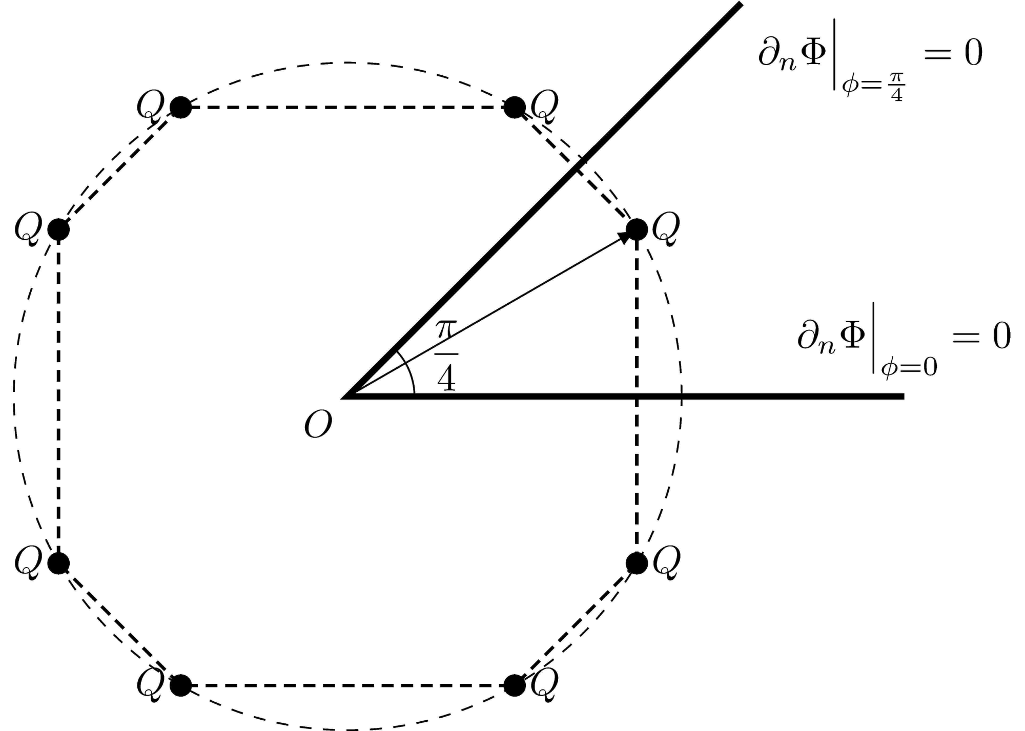
Figure 3: The positions of the charge $Q$ and image charges for $n=4$ with Neumann boundary condition.

It’s just that all the image charges and source charges have the same sign at this time. So

$$\begin{array}{}\text{(24)}& {\varphi }_i=\left[\frac{i}{2}\right]\frac{2\pi }{n}+(-1{)}^{i+1}{\varphi }_0,(i=1,2,\dots ,2n).\end{array}$$

and

$$\begin{array}{}\text{(25)}& \mathrm{\Phi }(r,\varphi ,z)=\frac{Q}{4\pi {ϵ}_0}\sum _{i=1}^{2n}\frac{1}{\sqrt{r^2+r_0^2+z^2-2r{r}_0\cos (\varphi -{\varphi }_i)}}.\end{array}$$

2.2. General case: $\alpha$ can be any value

In order to satisfy the Neumann boundary condition ${\partial }_n\mathrm{\Phi }=0$ , it is only necessary to modify the eigenfunction in the $\varphi$ direction . One thing that needs to be noted is the situation of $k=0$ cannot be thrown away, then

$$\psi (\varphi )=\cos \left(\frac{k\pi }{\alpha }\varphi \right),m=\frac{k\pi }{\alpha }(k=0,1,2,\dots )$$

So the general solution must also be modified,

$$\begin{array}{rl}\mathrm{\Phi }(r,\varphi ,z)& =\sum _{k=0}^{\mathrm{\infty }}{\int }_0^{\mathrm{\infty }}\mathrm{d}\mu a_{k\mu }{\mathrm{\Phi }}_{k\mu }(r,\varphi ,z)\\ & =\{\begin{array}{ll}{\displaystyle \sum _{k=0}^{\mathrm{\infty }}{\int }_0^{\mathrm{\infty }}\mathrm{d}\mu A_{k\mu }{I}_{k\pi /\alpha }(\mu r)\cos \left(\mu z\right)\cos \left(\frac{k\pi }{\alpha }\varphi \right),}& r<r_0\\ {\displaystyle \sum _{k=0}^{\mathrm{\infty }}{\int }_0^{\mathrm{\infty }}\mathrm{d}\mu B_{k\mu }{K}_{k\pi /\alpha }(\mu r)\cos \left(\mu z\right)\cos \left(\frac{k\pi }{\alpha }\varphi \right),}& r>r_0\end{array}\end{array}$$

The coefficients can be solved using the same method as before:

$$\{\begin{array}{l}{\displaystyle A_{0\mu }=\frac{Q}{\alpha {ϵ}_0\pi }{K}_0(\mu r_0)}\\ {\displaystyle B_{0\mu }=\frac{Q}{\alpha {ϵ}_0\pi }{I}_0(\mu r_0)}\end{array},\{\begin{array}{l}{\displaystyle A_{k\mu }=\frac{2Q}{\alpha {ϵ}_0\pi }\cos \left(\frac{k\pi {\varphi }_0}{\alpha }\right)K_{k\pi /\alpha }(\mu r_0)}\\ {\displaystyle A_{k\mu }=\frac{2Q}{\alpha {ϵ}_0\pi }\cos \left(\frac{k\pi {\varphi }_0}{\alpha }\right)I_{k\pi /\alpha }(\mu r_0)}\end{array}(k=1,2,\dots )$$

Thus, the final result of the electric potential is

$$\begin{array}{}\text{(26)}& \mathrm{\Phi }(r,\varphi ,z)=\frac{Q}{\alpha {ϵ}_0\pi \sqrt{r_{0}r}}\{\frac{1}{2}{Q}_{-\frac{1}{2}}\left(\frac{r^2+r_0^2+z^2}{2r_{0}r}\right)+\sum _{k=1}^{\mathrm{\infty }}{Q}_{\frac{k\pi }{\alpha }-\frac{1}{2}}\left(\frac{r^2+r_0^2+z^2}{2r_{0}r}\right)\cos \left(\frac{k\pi {\varphi }_0}{\alpha }\right)\cos \left(\frac{k\pi \varphi }{\alpha }\right)\}.\end{array}$$

2.3. Prove they are equivalent if $\alpha =\pi /n$

Also use formula $\text{(22)}$,

$$\begin{array}{rl}& \sum _{k=1}^{2n}\frac{1}{\sqrt{\xi -\cos (\varphi -{\varphi }_k)}}\\ =& \sqrt{2r_{0}r}\sum _{k=1}^{2n}\frac{1}{\sqrt{r^2+r_0^2+z^2-2r_{0}r\cos (\varphi -{\varphi }_k)}}\\ =& \sqrt{2r_{0}r}\{\frac{1}{\pi \sqrt{r{r}_0}}\sum _{k=1}^{2n}{Q}_{-\frac{1}{2}}\left(\frac{r^2+r_0^2+z^2}{2r_{0}r}\right)+\frac{2}{\pi \sqrt{r{r}_0}}\sum _{m=1}^{\mathrm{\infty }}{\cos }^{m(\varphi -{\varphi }_k)}{Q}_{m-\frac{1}{2}}\left(\frac{r^2+r_0^2+z^2}{2r{r}_0}\right)\}\\ =& \frac{4\sqrt{2}n}{\pi }\{\frac{1}{2}{Q}_{-\frac{1}{2}}(\xi )+\sum _{m=1}^{\mathrm{\infty }}{Q}_{m-\frac{1}{2}}(\xi )\sum _{k=1}^{\mathrm{\infty }}\frac{\cos [\varphi -\left[{\displaystyle \frac{k}{2}}\right]{\displaystyle \frac{2\pi }{n}}+(-1{)}^k{\varphi }_0]}{2n}\}.\end{array}$$

For the summation of $k$ on the right side, it can be calculated directly

$$\frac{1}{2n}\sum _{k=1}^{2n}\cos \left[m(\varphi -\left[\frac{k}{2}\right]\frac{2\pi }{n}+(-1{)}^k{\varphi }_0)\right]=\{\begin{array}{ll}0,& ({\displaystyle \frac{m}{n}}\ne p)\\ \cos \left(m\varphi \right)\cos \left(m{\varphi }_0\right),& ({\displaystyle \frac{m}{n}}=p)\end{array}$$

So

$$\begin{array}{}\text{(27)}& \begin{array}{rl}& \sum _{k=1}^{2n}\frac{1}{\sqrt{\xi -\cos (\varphi -{\varphi }_k)}}\\ =& \frac{4\sqrt{2}n}{\pi }\{\frac{1}{2}{Q}_{-\frac{1}{2}}(\xi )+\sum _{k=1}^{\mathrm{\infty }}{Q}_{nk-\frac{1}{2}}\left(\xi \right)\cos \left(nk{\varphi }_0\right)\cos \left(nk\varphi \right)\}.\end{array}\end{array}$$

This is the result given after the two solutions $\text{(25)}$ and $\text{(26)}$ are equivalent.

3. Problem with mixed boundary condition

The problem with mixed boundary condition can also be solved. See the following results.

3.1. Special case: $\alpha =\pi /2n$

Note that this is different from the previous two cases. When $\alpha =\pi /(2n-1)$, the method of images is no longer valid. So we just discuss the case when $\alpha =\pi /2n$, see following example

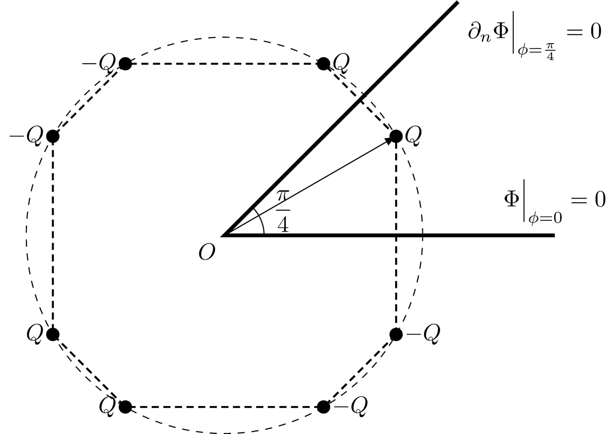
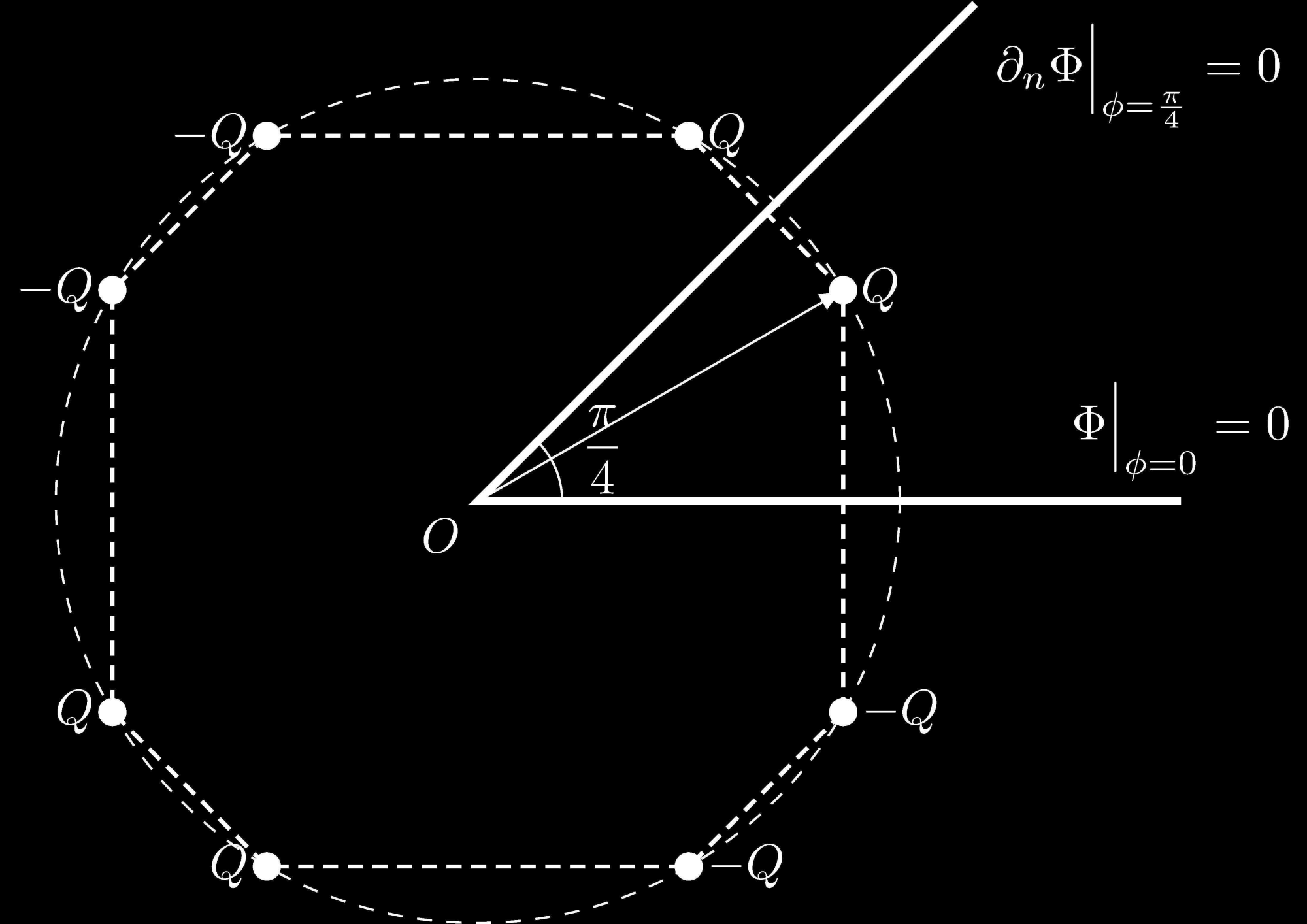Figure 4: The positions of the charge $Q$ and image charges for $n=4$ with mixed boundary condition.

So

$$\begin{array}{}\text{(28)}& {\varphi }_i=\left[\frac{i}{2}\right]\frac{\pi }{n}+(-1{)}^{i+1}{\varphi }_0.(i=1,2,\dots ,4n),\end{array}$$

and the electric potential is

$$\mathrm{\Phi }(r,\varphi ,z)=\frac{Q}{4\pi {ϵ}_0}\sum _{k=1}^{2n}\{\frac{(-1{)}^{k+1}}{\sqrt{r^2+r_0^2+z^2-2r{r}_0\cos (\varphi -{\varphi }_{2k-1})}}+\frac{(-1{)}^{k+1}}{\sqrt{r^2+r_0^2+z^2-2r{r}_0\cos (\varphi -{\varphi }_{2k})}}\}.$$

3.2. General case: $\alpha$ can be any value

Also modify the eigenfunction in the $\varphi$ direction by using

$$\psi (\varphi )=\sin \left(\frac{(2k-1)\pi }{2\alpha }\varphi \right),m=\frac{(2k-1)\pi }{2\alpha }(k=1,2,\dots ).$$

The general solution is

$$\begin{array}{rl}\mathrm{\Phi }(r,\varphi ,z)& =\sum _{k=1}^{\mathrm{\infty }}{\int }_0^{\mathrm{\infty }}\mathrm{d}\mu a_{k\mu }{\mathrm{\Phi }}_{k\mu }(r,\varphi ,z)\\ & =\{\begin{array}{ll}{\displaystyle \sum _{k=1}^{\mathrm{\infty }}{\int }_0^{\mathrm{\infty }}\mathrm{d}\mu A_{k\mu }{I}_{\frac{(2k-1)\pi }{2\alpha }}(\mu r)\cos \left(\mu z\right)\sin \left(\frac{(2k-1)\pi }{2\alpha }\varphi \right),}& r<r_0\\ {\displaystyle \sum _{k=1}^{\mathrm{\infty }}{\int }_0^{\mathrm{\infty }}\mathrm{d}\mu B_{k\mu }{K}_{\frac{(2k-1)\pi }{2\alpha }}(\mu r)\cos \left(\mu z\right)\sin \left(\frac{(2k-1)\pi }{2\alpha }\varphi \right),}& r>r_0\end{array}\end{array}$$

And the coefficients are

$$\begin{array}{}\text{(29)}& \{\begin{array}{l}{\displaystyle A_{k\mu }=\frac{2Q}{\alpha {ϵ}_0\pi }\sin \left(\frac{(2k-1)\pi }{2\alpha }{\varphi }_0\right)K_{\frac{(2k-1)\pi }{2\alpha }}(\mu r_0),}\\ {\displaystyle B_{k\mu }=\frac{2Q}{\alpha {ϵ}_0\pi }\sin \left(\frac{(2k-1)\pi }{2\alpha }{\varphi }_0\right)I_{\frac{(2k-1)\pi }{2\alpha }}(\mu r_0).}\end{array}\end{array}$$

And the final result is

$$\begin{array}{}\text{(30)}& \mathrm{\Phi }(r,\varphi ,z)=\frac{Q}{\alpha {ϵ}_0\pi \sqrt{r_{0}r}}\sum _{k=1}^{\mathrm{\infty }}{Q}_{\frac{(2k-1)\pi }{2\alpha }-\frac{1}{2}}\left(\frac{r^2+r_0^2+z^2}{2r_{0}r}\right)\sin \left(\frac{(2k-1)\pi {\varphi }_0}{2\alpha }\right)\sin \left(\frac{(2k-1)\pi \varphi }{2\alpha }\right).\end{array}$$

3.3. Prove they are equivalent if $\alpha =\pi /2n$

Also use formula $\text{(22)}$,

$$\begin{array}{rl}& \sum _{k=1}^{2n}\{\frac{(-1{)}^{k+1}}{\sqrt{\xi -\cos (\varphi -{\varphi }_{2k-1})}}+\frac{(-1{)}^{k+1}}{\sqrt{\xi -\cos (\varphi -{\varphi }_{2k})}}\}\\ =& \sqrt{2r_{0}r}\{\sum _{k=1}^{2n}\frac{(-1{)}^{k+1}}{\sqrt{r^2+r_0^2+z^2-2r_{0}r\cos (\varphi -{\varphi }_{2k-1})}}+\sum _{k=1}^{2n}\frac{(-1{)}^{k+1}}{\sqrt{r^2+r_0^2+z^2-2r_{0}r\cos (\varphi -{\varphi }_{2k})}}\}\\ =& \frac{2\sqrt{2}}{\pi }\sum _{m=1}^{\mathrm{\infty }}{Q}_{m-\frac{1}{2}}(\xi )\{\sum _{k=1}^{2n}(-1{)}^{k+1}{\cos }^{m(\varphi -{\varphi }_{2k-1})}+\sum _{k=n}^{2n}(-1{)}^{k+1}{\cos }^{m(\varphi -{\varphi }_{2k})}\}\\ =& \frac{4\sqrt{2}}{\pi }\sum _{m=1}^{\mathrm{\infty }}{Q}_{m-\frac{1}{2}}(\xi )\cos (m{\varphi }_0-\frac{m\pi }{2n})\sum _{k=1}^{2n}(-1{)}^{k+1}\cos [m\varphi -\frac{(2k-1)m\pi }{2n}].\end{array}$$

Calculate the second sum of the above equation,

$$\begin{array}{r}\sum _{k=1}^{2n}(-1{)}^{k+1}\cos [m\varphi -\frac{(2k-1)m\pi }{2n}]=\{\begin{array}{ll}{\displaystyle -2n\cos (m\varphi +\frac{m\pi }{2n}),}& ({\displaystyle \frac{m}{n}}=2p-1)\\ 0,& ({\displaystyle \frac{m}{n}}=2p-1)\end{array}\end{array}$$

then

$$\begin{array}{rl}& \sum _{k=1}^{2n}\{\frac{(-1{)}^{k+1}}{\sqrt{\xi -\cos (\varphi -{\varphi }_{2k-1})}}+\frac{(-1{)}^{k+1}}{\sqrt{\xi -\cos (\varphi -{\varphi }_{2k})}}\}\\ =& -\frac{8\sqrt{2}n}{\pi }\sum _{p=1}^{\mathrm{\infty }}{Q}_{(2p-1)n-\frac{1}{2}}(\xi )\cos ((2p-1)n{\varphi }_0-\frac{(2p-1)\pi }{2})\cos ((2p-1)n\varphi +\frac{(2p-1)\pi }{2}).\end{array}$$

That is,

$$\begin{array}{}\text{(31)}& \begin{array}{rl}& \sum _{k=1}^{2n}\{\frac{(-1{)}^{k+1}}{\sqrt{\xi -\cos (\varphi -{\varphi }_{2k-1})}}+\frac{(-1{)}^{k+1}}{\sqrt{\xi -\cos (\varphi -{\varphi }_{2k})}}\}\\ =& \frac{8\sqrt{2}n}{\pi }\sum _{k=1}^{\mathrm{\infty }}{Q}_{(2p-1)n-\frac{1}{2}}(\xi ){\sin }^{(2p-1)n{\varphi }_0}{\sin }^{(2p-1)n\varphi },\end{array}\end{array}$$

which is what we want to verify.

4. Appendix: Prove the integral formula

We used $\text{(16)}$ in our previous calculation without proof, and now we prove it. With Sonine-Gegenbauer integral

$${\int }_0^{\pi }\frac{t^{\nu }{J}_{\nu }(t\sqrt{a^2+b^2-2ab\cos \theta })}{(a^2+b^2-2ab\cos \theta {)}^{\nu /2}}{\sin }^{2\nu }\theta \mathrm{d}\theta =\frac{\pi \mathrm{\Gamma }(2\nu )}{2^{\nu -1}\mathrm{\Gamma }(\nu )}\frac{J_{\nu }(at)}{a^{\nu }}\frac{J_{\nu }(bt)}{b^{\nu }},$$

we calculate the integration of $J_{\nu }(ax)J_{\nu }(bx){\mathrm{e}}^{-cx}$,

$$\begin{array}{rl}& \frac{\pi \mathrm{\Gamma }(2\nu )}{2^{\nu -1}\mathrm{\Gamma }(\nu )}\frac{1}{a^{\nu }{b}^{\nu }}{\int }_0^{\mathrm{\infty }}{J}_{\nu }(at)J_{\nu }(bt){\mathrm{e}}^{-ct}\mathrm{d}t\\ =& {\int }_0^{\mathrm{\infty }}({\int }_0^{\pi }\frac{t^{\nu }{J}_{\nu }(t\sqrt{a^2+b^2-2ab\cos \theta })}{(a^2+b^2-2ab\cos \theta {)}^{\nu /2}}{\sin }^{2\nu }\theta \mathrm{d}\theta ){\mathrm{e}}^{-ct}\mathrm{d}t\\ =& {\int }_0^{\pi }\frac{{\sin }^{2\nu }\theta }{(a^2+b^2-2ab\cos \theta {)}^{\nu /2}}({\int }_0^{\mathrm{\infty }}{t}^{\nu }{J}_{\nu }(t\sqrt{a^2+b^2-2ab\cos \theta }){\mathrm{e}}^{-ct}\mathrm{d}t)\mathrm{d}\theta \end{array}$$

Then use the following two integral formulas,

$${\int }_0^{\mathrm{\infty }}{\mathrm{e}}^{-ax}{J}_{\nu }(bx)x^{\nu }\mathrm{d}x=\frac{b^{\nu }\mathrm{\Gamma }(2\nu +1)}{2^{\nu }\mathrm{\Gamma }(\nu +1)}\frac{1}{(a^2+b^2{)}^{\nu +1/2}},$$

and

$$\begin{array}{rl}& {\int }_0^{\mathrm{\infty }}{t}^{\nu }{J}_{\nu }(t\sqrt{a^2+b^2-2ab\cos \theta }){\mathrm{e}}^{-ct}\mathrm{d}t\\ =& \frac{(\sqrt{a^2+b^2-2ab\cos \theta }{)}^{\nu }\mathrm{\Gamma }(2\nu +1)}{2^{\nu }\mathrm{\Gamma }(\nu +1)}\frac{1}{(c^2+a^2+b^2-2ab\cos \theta {)}^{\nu +1/2}}.\end{array}$$

Substituting into the above formula, we can get

$$\begin{array}{rl}\frac{\pi \mathrm{\Gamma }(2\nu )}{2^{\nu -1}\mathrm{\Gamma }(\nu )}\frac{1}{a^{\nu }{b}^{\nu }}{\int }_0^{\mathrm{\infty }}{J}_{\nu }(at)J_{\nu }(bt){\mathrm{e}}^{-ct}\mathrm{d}t& =\frac{\mathrm{\Gamma }(2\nu +1)}{2^{\nu }\mathrm{\Gamma }(\nu +1)}{\int }_0^{\pi }\frac{{\sin }^{2\nu }\theta }{(c^2+a^2+b^2-2ab\cos \theta {)}^{\nu +1/2}}\mathrm{d}\theta \\ & =\frac{\mathrm{\Gamma }(2\nu +1)}{2^{\nu }\mathrm{\Gamma }(\nu +1)}\frac{2^{\nu +1/2}}{(2ab{)}^{\nu +1/2}}{Q}_{\nu -\frac{1}{2}}\left(\frac{c^2+a^2+b^2}{2ab}\right).\end{array}$$

So

$${\int }_0^{\mathrm{\infty }}{J}_{\nu }(at)J_{\nu }(bt){\mathrm{e}}^{-ct}\mathrm{d}t=\frac{1}{\pi \sqrt{ab}}{Q}_{\nu -\frac{1}{2}}\left(\frac{a^2+b^2+c^2}{2ab}\right).$$

Following the derivation in this post, we can give the cylindrical coordinate expansion of Green’s function in another form (like $\text{(22)}$):

$$\frac{1}{|\mathbf{x}-{\mathbf{x}}^{\prime }|}=\frac{2}{\pi }\sum _{m=-\mathrm{\infty }}^{\mathrm{\infty }}{\int }_0^{\mathrm{\infty }}\mathrm{d}k{\mathrm{e}}^{im(\varphi -{\varphi }^{\prime })}{\cos }^{k(z-z^{\prime })}{I}_m(k{r}_{<})K_m(k{r}_{>}).$$

By choosing different constant forms when separating variables, we can get another expansion form of Green’s function in cylindrical coordinates:

$$\frac{1}{|\mathbf{x}-{\mathbf{x}}^{\prime }|}=\sum _{m=-\mathrm{\infty }}^{\mathrm{\infty }}{\int }_0^{\mathrm{\infty }}\mathrm{d}k{e}^{im(\varphi -{\varphi }^{\prime })}{J}_m(kr)J_m(k{r}^{\prime }){\mathrm{e}}^{-k(z_{>}-z_{<})}.$$

Since they are the same Green’s function, the two expansion forms are equivalent. The only difference lies in the selection of constants when separating variables. Note that $e^{im(\varphi -{\varphi }^{\prime })}$ is pairwise orthogonal when $m$ is different. By comparing their coefficients, we can easily get:

$${\int }_0^{\mathrm{\infty }}\mathrm{d}k\frac{2}{\pi }{K}_m(k{r}_{>})I_m(k{r}_{<}){\cos }^{k(z-z^{\prime })}={\int }_0^{\mathrm{\infty }}\mathrm{d}k{J}_m(kr)J_m(k{r}^{\prime })e^{-k(z_{>}-z_{<})}.$$

Thus,

$${\int }_0^{\mathrm{\infty }}{K}_{\nu }(ax)I_{\nu }(bx)\cos \left(cx\right)\mathrm{d}x=\frac{1}{2\sqrt{ab}}{Q}_{\nu -\frac{1}{2}}\left(\frac{a^2+b^2+c^2}{2ab}\right).$$

This is exactly $\text{(16)}$.

1. Zwillinger, D. (Ed.). Table of integrals, series, and products (8th ed.). Academic Press. p. 726. (2014) ↩︎